This is a template that exists within the Community Solutions add-on for Google Sheets, but there was no Excel version. With the blessing of the original creator @jono, here is an Excel version.
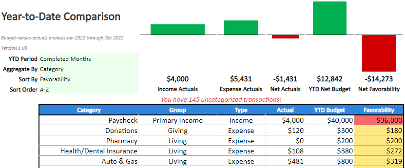
This Year to Date Comparison sheet provides budget versus actual analysis for the year to date period. The sheet is very simple and easy to use. It works for the current year.
Follow these instructions to copy the downloaded template into your Excel workbook and to connect the formula references to your local workbook data.
Usage
Aggregate By: Options are Category or Group.
Sort By: The report can be sorted by any of the columns.
Sort Order: The report can be sorted A to Z or Z to A.
The sheet summarizes in your actual Transactions by Category and Group from the Transactions sheet for the year to date period.
The sheet works best if you are using a Categories sheet that includes budgets by month. The Foundation template includes this. If you don’t have a Categories sheet with budgets by month starting in Jan of this year, then you won’t have any YTD Budget data.
If a category or group doesn’t have an actual amount or a budget amount, it won’t appear in the report. Categories that are set to Hide won’t appear either.
I deliberately avoided creating any links/connections on this template, so you can skip the required step for changing them (as you’ve found, the ‘Edit Links’ button is greyed out since there’s nothing that can be edited). The formulas should find the data in your template as long as you have relatively normal Transactions and Categories sheets.
You continue to lead the charge to template parity, @jpfieber. So cool that you can turn a community request into a robust solution in just five days. Also really thoughtful of you to share credit with @jono, the creator of the Sheets version.
The Tiller team is excited to award you $300 as part of the Tiller Builder Rewards Program for building and documenting this template for the Tiller community.
@jpfieber I can’t figure out how to update this for my new 2023 Tiller workbook. The dates are not picking up 2023 and therefore no data. Any suggestions on where it’s broke? Should I download again and add to my new 2023 workbook?
Just installed this add-on. Thank you for building it. On the top right corner, is it possible to add a filter to filter out specific categories. One of my categories is Savings contributions which is not exactly an expense but it is shows up in the ‘Expense Actuals’
Suddenly the Year-to-Date Comparison stopped working. I am getting #ref! in Columns T U AB AE and no comparison to Budget. All the actual results are OK. What do you think happened?
I would suspect something got typed into a cell on that sheet and is preventing a formula from ‘spilling’ it’s data. I’d suggest trying to select the range O3:W40 and hit the delete key to delete anything in those cells. Do the same for the range Y3:AE04. If that doesn’t do it, I’d probably just start fresh with the template, since you won’t be losing much in the way of data. Delete the existing sheet and then recopy from the original download.
I just re-added it to my workbook and it’s working, so I don’t think the problem lies with the template itself, it must be something different about your workbook/data. Does your column W show a list of ranges? For example, mine shows:
E2:O2
E3:O3
E4:O4
E5:O5
E6:O6
E7:O7
E8:O8
E9:O9
E10:O10
E11:O11
E12:O12
E13:O13
E14:O14
E15:O15
E16:O16
E17:O17
Etc.
The sheet is getting these from your Categories sheet. If it can’t find these, that would break stuff.
Ahh, good sleuthing. Apparently the CHAR(64+K16) method of converting a column number to a letter only works with one letter. Since yours expanded to two letters, we didn’t get what we’re looking for. To fix this, replace L16 with =SUBSTITUTE(ADDRESS(1, K16, 4), "1", "") and L17 with =SUBSTITUTE(ADDRESS(1, K17, 4), "1", ""). This formula will work with single or double letters. I’ll update the template so future users don’t get bothered by this (and bump the version number to 1.01), thanks for helping track it down!